Lab 6

Get the code

Find the Lab 6 code in the class repository.

$ ls
README.md  classes/   labs/      scripts/
$ ls labs/lab6
README    cpp/      julia/    python/   rust/
$ ls labs/lab6/python
en.gp     ft.gp     traj.gp   well.dat  well.py

The instructions here focus on Python, but you may carry out the comparable steps in C++, Julia, or Rust.

Harmonic oscillator trajectory

The program well.py simulates a particle of mass \(\mathsf{m}\) moving in a quadratic well of stiffness \(\mathsf{K}\). The time evolution is carried out using the standard Velocity Verlet algorithm, and the simulation runs over several multiples of the oscillator period \(P = \mathsf{2 \pi/ \sqrt{K/m}}\). The time step is chosen to be \(\mathsf{\Delta t} = P/200\).

The gnuplot scripts traj.gp and en.gp demonstrate the oscillatory behaviour and confirm the conservation of energy.

$ python3 well.py > well.dat
runtime = 157.07963267948966
 period = 6.283185307179586
 freq = 0.15915494309189535

Running simulation...
Running simulation...
Done.
Computing discrete Fourier Transforms...
Done cos.
Done sin.

$ gnuplot -persist traj.gp
$ gnuplot -persist en.gp

Discrete Fourier transforms

The output to the file well.dat is broken into two blocks. The first block lists the trajectory data in \(\mathsf{t}, \mathsf{x}, \mathsf{v}, \mathsf{E}\) format. The second block lists the \(\textsf{cos}\) and \(\textsf{sin}\) discrete Fourier transforms (in the second and third columns) as a function of frequency (in the first column).

$ head -n 5 well.dat
000000   0.999507  -0.031408   0.500000
031416   0.998027  -0.062785   0.500000
062832   0.995562  -0.094101   0.499999
094248   0.992114  -0.125323   0.499998
125664   0.987687  -0.156422   0.499997
$ tail -n 5 well.dat
799158   0.214164   0.001484
805524   0.211001   0.001170
811890   0.208605   0.000867
818256   0.206926   0.000574
824622   0.205932   0.000285
$ head -n 5006 well.dat | tail -n 12
891137   0.988677   0.150038   0.499997
922553   0.992903   0.118912   0.499998
953969   0.996149   0.087668   0.499999
985385   0.998411   0.056337   0.500000
016801   0.999689   0.024951   0.500000
048217   0.999979  -0.006460   0.500000


000000   0.205602   0.000000
006366   0.205932  -0.000285
012732   0.206926  -0.000574
019099   0.208605  -0.000867

The corresponding spectum is strongly peaked at the natural frequency \(\mathsf{\nu \doteq 0.159}\).

$ gnuplot -persist ft.gp

Stochastic evolution

We now want to include some random behaviour in the time evolution of the particle. In particular, we imagine that the particle is immersed in a fluid in thermal equilibrium at temperature \(T\). The fluid provides both a drag on the particle and a random stochastic force due to the fluctuating impact of the fluid molecules.

Start by building your own high-quality random number generator. Blum Blum Shub (BBS) is a famous scheme that generates one random bit per iteration. Implement BBS with the parameters \(\mathsf{p} = \mathsf{2\,888\,799\,659}`\) and \(\mathsf{q} = \mathsf{3\,694\,568\,831}\), say, so that the modulus is \(\mathsf{M} = \mathsf{pq} = \mathsf{10\,672\,869\,179\,144\,828\,629}\). The seed \(\mathsf{x_0}\) must be coprime to \(\mathsf{M}\). Let’s choose \(\mathsf{x_0} = \mathsf{326\,694\,129}\).

Write a function R() that returns a random number drawn uniformly from the interval \(\mathsf{[0,1)}\). You’ll have to generate 52 bits (the width of the mantissa) to populate one double-precision floating-point value.

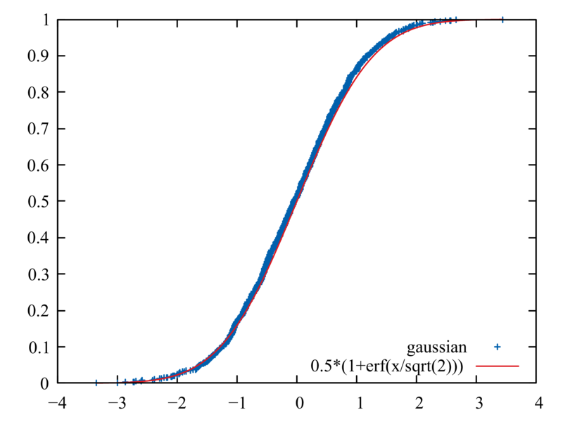
Then write another function RN() that returns a random number drawn from the normal (i.e., Guassian) distribution with zero mean and unit variance. You should use the Box-Muller trick.

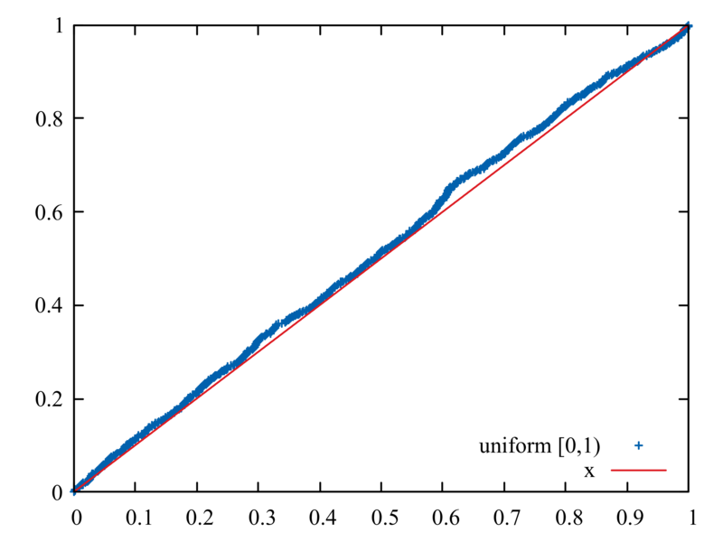
The following is a good way to test that your generators are unbiased and performing correctly. Produce 1000 random numbers each with R() and RN(), arranged in ascending order; compare each set to its corresponding cumulative probability distribution

import math
import sys
import struct
print("Testing random number generator", file=sys.stderr)
r=[]
rr=[]
for n in range(1000):
    r.append(R())
    rr.append(RN())
r.sort()
rr.sort()
f = open("rng-test.dat","w")
for n in range(len(r)):
    f.write("{:8.4} {:15.8} {:15.8}\n".format((n+0.5)/len(r),r[n],rr[n]))
f.close()
exit()

set key bottom right
plot[][0:1] "rng-test.dat" using 2:1 title "uniform [0,1)", x
pause -1
plot[][:1] "rng-test.dat" using 3:1 title "gaussian", 0.5*(1+erf(x/sqrt(2)))
pause -1

Langevin equation

Rework the simulation to accommodate an expanded set of forces, including \(\mathsf{F}_\textsf{drag} = - \mathsf{\gamma v}\) and \(\mathsf{F}_\textsf{thermal}\) in addition to the Hooke’s law force \(\mathsf{F(x)} = -\mathsf{V'(x)} = -\mathsf{Kx}\). Use the following Verlet-like update scheme:

\[\begin{aligned} \mathsf{x_{n+1}} &= \mathsf{x_n} + \mathsf{bv_n\Delta t} + \mathsf{\frac{b(\Delta t)^2}{2m}F(x_n)} + \mathsf{\frac{b \Delta t}{2m}\beta_{n+1}}, \\ \mathsf{v_{n+1}} &= \mathsf{v_n} + \mathsf{\frac{\Delta t}{2m} \bigl(F(x_n) + F(x_{n+1})\bigr)} - \mathsf{\frac{\gamma}{m}\bigl(x_{n+1}-x_n\bigr)} + \mathsf{\frac{1}{m}\beta_{n+1}}. \end{aligned}\]

Here, \(\mathsf{b} = \textsf{exp}(-\mathsf{\gamma \Delta t/2m})\) and each \(\mathsf{\beta} = \sqrt{\mathsf{2 \gamma k_B T \Delta t}}\,\xi\) is a random value with \(\xi\) representing the result of the function call RN().

Perform several runs in which you systematically ramp up the damping from zero. The temperature can be fixed at the value \(\mathsf{k_BT} = \mathsf{1/2}\), consistent with initial conditions and the energy predicted by equipartition. Make a plot showing the resulting changes in the Fourier transform peak.