Lab 2
Get the code
Find the Lab 2 code in the class repository.
$ ls
README.md  classes/   labs/      scripts/
$ ls labs/lab2
README    cpp/      julia/    python/   rust/
$ ls labs/lab2/cpp
curves.cpp   makefile     triples.cpp  view-trip.gp
The instructions here focus on C++, but you may carry out the comparable steps in Julia, Python, or Rust. You only need to submit your solutions for a single programming language.
Ordered tuples
The lab2 directory contains a short C++ program named
triples.cpp that outputs all strictly ordered triples of the
integers 0 to 6 (inclusive). The make command invokes the compiler,
which creates an executable named triples.
$ make triples
g++ -o triples triples.cpp -O -ansi -pedantic -Wall
$ ./triples
(0,1,2)
(0,1,3)
(0,2,3)
(1,2,3)
.
.
.
(1,5,6)
(2,5,6)
(3,5,6)
(4,5,6)
Modify the program so that instead it counts the number of such triples. Generalize to integers \(\mathsf{0}, \mathsf{1}, \ldots, \mathsf{N}\), and output the results in two-column format for all values of \(\mathsf{N}\) from 2 to 10. You should be able to reproduce the following.
$ make triples
g++ -o triples triples.cpp -O -ansi -pedantic -Wall
 $ ./triples
     2           1
     3           4
     4          10
     5          20
     6          35
     7          56
     8          84
     9         120
    10         165
$ ./triples > trip.dat
$ gnuplot view-trip.gp
(If your plot doesn’t persist, you may have to type
gnuplot -p view-trip.gp. Whether the -p flag is required
depends on which operating system you’re running. Alternatively, you
can add pause -1 as the last line of your gnuplot script.)
Redirection from stdout to a file via > trip.dat is a shell feature
and not specific to C++, which is to say that you can do all of the
following:
$ cd ../julia
$ julia triples.jl > trip.dat
$ cd ../python
$ python3 triples.py > trip.dat
$ cd ../rust
$ rustc triples.rs
$ ./triples > trip.dat
$ cd ../cpp
Using your solution to triples.cpp as a template, create a program
file quadruples.cpp that writes three columns of data:
\(\mathsf{N}\) from 0 to 99, the number of weakly ordered
quadruples \(\mathsf{(i,j,k,l)}\) formed from the integers
\(\mathsf{0}\) through \(\mathsf{N}\), and how many of the sums
\(\mathsf{i^2 + j^2 + k^2 + l^2}\) are perfect squares.
(Strict ordering of \(\mathsf{i}\), \(\mathsf{j}\),
\(\mathsf{k}\), and \(\mathsf{l}\) implies that
\(\mathsf{i < j < k < l}\). Weak ordering implies
that \(\mathsf{i \le j \le k \le l}\).)
$ make quadruples
g++ -o quadruples quadruples.cpp -O -ansi -pedantic -Wall
$ ./quadruples
     0           1           1
     1           5           3
     2          15           6
     3          35           8
     4          70          14
     5         126          18
     .           .           .
     .           .           .
     .           .           .
    97     4082925       15689
    98     4249575       16213
    99     4421275       16462
Determine whether an integer is a perfect square by whatever means. You
may want to use std::sqrt from the cmath library in combination
with integer casting.
Following view-trip.gp, compose a gnuplot script file view-quad.gp
that plots the number of perfect squares alongside the 3rd- and
4th-order polynomial fits to the data.
Selection rules
The hydrogen atom consists of a single electron orbiting a positively charged nucleus. The electron can exist only in discrete orbitals characterized by the radial quantum number \(\mathsf{n} = \mathsf{1}, \mathsf{2}, \mathsf{3}, \ldots\) and the angular momentum quantum numbers \(\mathsf{l} = \mathsf{0}, \mathsf{1}, \mathsf{2}, \ldots, \mathsf{n-1}\) and \(\mathsf{m} = \mathsf{-l}, \ldots, \mathsf{-1}, \mathsf{0}, \mathsf{1}, \ldots, \mathsf{l}\). The energy of each orbital, \(\mathsf{E_n} = \mathsf{-(13.6\,\textsf{eV})/n^2}\), is a function of the radial quantum number alone. Hence, each energy level is \(\mathsf{g_n}\)-fold degenerate, where \(\mathsf{g_n} = \mathsf{\sum_{l=0}^{n-1} (2l+1)} = \mathsf{n^2}\). (In other words, there are \(\mathsf{g_n} = \mathsf{n^2}\) states having the same energy \(\mathsf{E_n}\).)
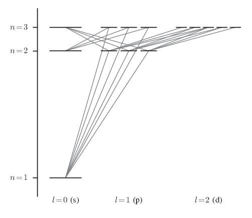
Transitions between orbitals can occur if the electron absorbs or emits a photon. But since a quantum of light has intrinsic angular momentum (1 in units of \(\mathsf{\hbar}\)), conservation laws put a strict limit on which atomic transitions are possible. This leads to the famous electric dipole selection rules: \(\mathsf{\Delta l} = \pm \mathsf{1}\) and \(\mathsf{\Delta m} = \mathsf{0}, \pm \mathsf{1}\). Allowed transitions between the various states with \(\mathsf{n} = \mathsf{1}, \mathsf{2}, \mathsf{3}\) are shown in the following diagram.
Complete the program selection.cpp so that it computes all possible
transitions of the form \(\mathsf{n_2} \to \mathsf{n_1}\) with
\(\mathsf{n_1} < \mathsf{n_2} \le \mathsf{20}\). Have the program
output the results in four columns indicating the initial and final
radial quantum numbers, the number of allowed pathways, the energy of
the emitted photon \(\mathsf{\Delta E} = \mathsf{E_2}
- \mathsf{E_1}\), and its wavelength \(\lambda = \mathsf{hc/\Delta
E}\) in nanometers. (Recall that \(\mathsf{hc}
= \mathsf{1240}\,\textsf{eV}\cdot\textsf{nm}\).)
$ make selection
g++ -o selection selection.cpp -O2 -ansi -pedantic -Wall -lm
$ ./selection | head -n5
 2->1         3            10.2         121.569
 3->1         3         12.0889         102.574
 3->2        15         1.88889         656.471
 4->1         3           12.75         97.2549
 4->2        15            2.55         486.275
Modify selection.cpp so that the spectral lines in the visible
spectrum, \(\mathsf{380}\,\textsf{nm} < \mathsf{\lambda}
< \mathsf{750}\,\textsf{nm}\), are marked with a lowercase v.
$ make selection
g++ -o selection selection.cpp -O2 -ansi -pedantic -Wall -lm
$ ./selection | head -n5
 2->1          3            10.2         121.569
 3->1          3         12.0889         102.574
 3->2v        15         1.88889         656.471
 4->1          3           12.75         97.2549
 4->2v        15            2.55         486.275
$ ./selection | grep v
 3->2v        15         1.88889         656.471
 4->2v        15            2.55         486.275
 5->2v        15           2.856         434.174
 6->2v        15         3.02222         410.294
 7->2v        15         3.12245         397.124
 8->2v        15          3.1875          389.02
 9->2v        15          3.2321         383.652
Spin sectors
Quantum particles have a property called spin, which is an intrinsic angular momentum. The spin of a particle is restricted to be a multiple of \(\mathsf{\hbar/2}\). In units where \(\mathsf{\hbar} = \mathsf{1}\), the spin is either an integer or an odd multiple of one half. Electrons have spin \(\mathsf{s=1/2}\).
The total spin \(S\) of a collection of electrons is determined by the angular momentum summation rule \(\mathsf{\tfrac{1}{2}} \otimes \mathsf{S} = \mathsf{(S-\tfrac{1}{2})} \oplus \mathsf{(S + \tfrac{1}{2})}\). The possible spin sectors for two, three, and four electrons are shown below.
The final line shows the general result for \(\mathsf{N}\) electrons. The coefficient \(\mathsf{C_S^{(N)}}\) denotes the number of states in a given spin sector. One can show that the total number of states in the singlet (\(\mathsf{S=0}\)) sector is
and that the total number of states—counting the \((\mathsf{2S+1})\)-fold degeracy—is
The \(\mathsf{2^N}\) result is just the number of ways to orient \(\mathsf{N}\) electrons either spin-up or spin-down.
Read over the file moments.cpp. It provides the skeleton of
a program that computes the coefficients \(\mathsf{C_S^{(N)}}\) and
displays them in a table. Determine how elements of the array
current (indexed by the integer \(\mathsf{2S}\)) should be
incremented in terms of the values in last. Accumulate the total
number of states into the variable num_states. The output of your
program should be identical to the following.
$ make moments
g++ -o moments moments.cpp -O2 -ansi -pedantic -Wall -lm
$ ./moments
         0    0.5      1    1.5      2    2.5      3    num
   +-------------------------------------------------+-------
  1|            1                                    |      2
  2|     1             1                             |      4
  3|            2             1                      |      8
  4|     2             3             1               |     16
  5|            5             4             1        |     32
  6|     5             9             5             1 |     64
  7|           14            14             6        |    128
  8|    14            28            20             7 |    256
  9|           42            48            27        |    512
 10|    42            90            75            35 |   1024
 11|          132           165           110        |   2048
 12|   132           297           275           154 |   4096
 13|          429           572           429        |   8192
 14|   429          1001          1001           637 |  16384
 15|         1430          2002          1638        |  32768
 16|  1430          3432          3640          2548 |  65536
   +-------------------------------------------------+-------
Write a function verify_singlet that computes
\(\mathsf{C_0^{(N)}}\) explicitly. Check its result against
last[0] for each even value of n from 2 to Nmax.