Lab 5
Get the code
Find the Lab 5 code in the class repository.
$    $ ls
README.md  classes/   labs/      scripts/
$ cd labs/lab5
README    cpp/      julia/    python/   rust/
$ ls labs/lab5/cpp
makefile   orbit.cpp  root.cpp   view1.gp   view3.gp
The instructions here focus on C++, but you may carry out the comparable steps in Julia, Python, or Rust.
Elliptic orbit
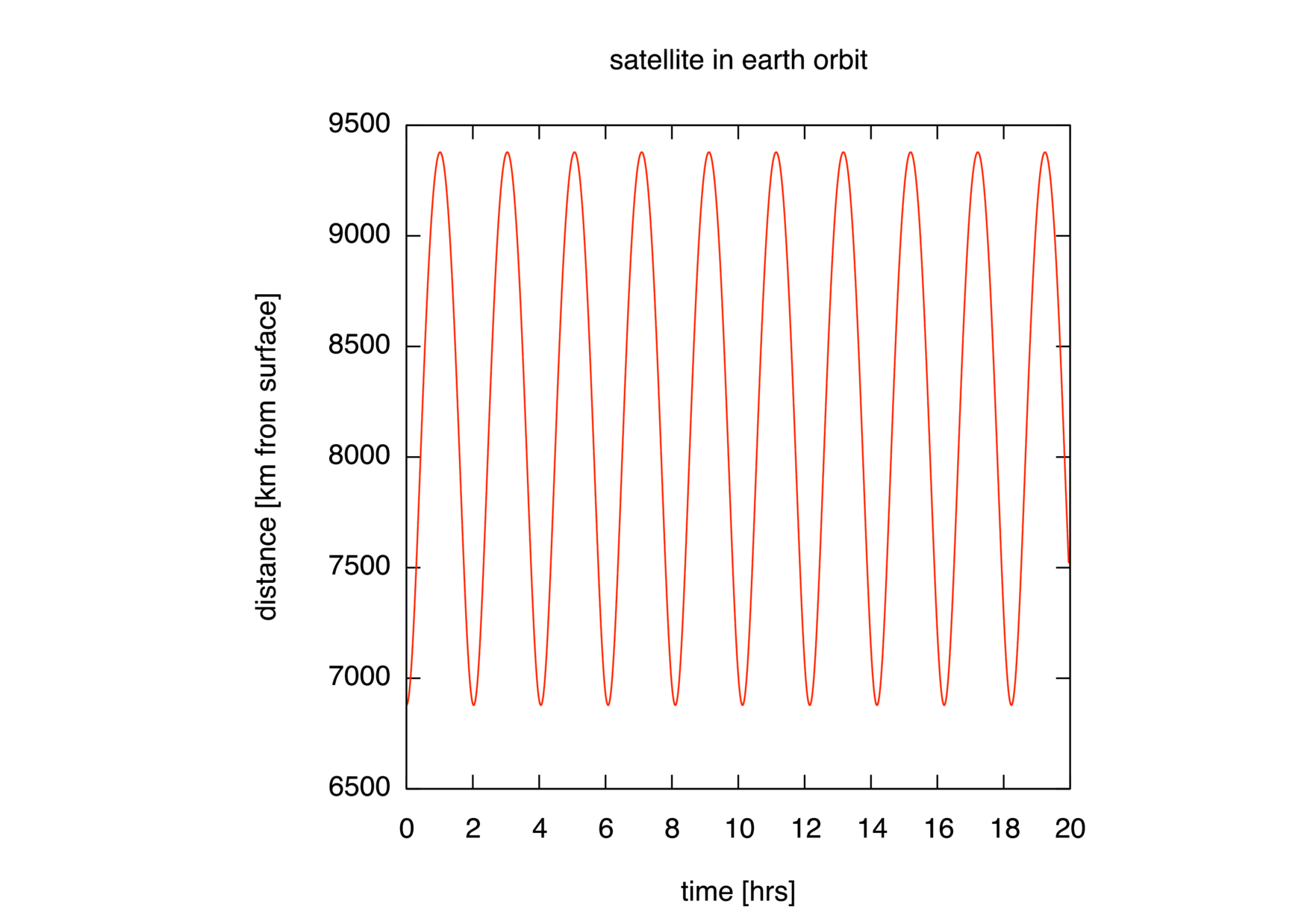
Consider a satellite orbiting the earth with period \(\mathsf{P}\) whose distances of closest and farthest approach are \(\mathsf{r_1}\) and \(\mathsf{r_2}\). The satellite’s path traces out an ellipse,
The formula above assumes polar coordinates \((\mathsf{r},\theta)\) in the lane of the orbit with the earth centred on one of the ellipse’s foci. The ratio
defines the eccentricity of the orbit; \(\mathsf{a}\) is the semi-major axis, and \(\mathsf{E}\) is the so-called eccentric anomaly.
Kepler worked out the following procedure for determining the location of the satellite at time \(\mathsf{t}\), as measured from the moment of closest approach:
Define the mean anomaly \(\mathsf{M} = \mathsf{2\pi t} / \mathsf{P}\).
Determine the eccentric anomaly \(\mathsf{E}\) by solving Kepler’s equation, \(\mathsf{M} = \mathsf{E} - \mathsf{e}\,\textsf{sin}\,\mathsf{E}\).
Compute the true anomaly \(\theta\) from the equation
\[\textsf{tan}\,\mathsf{\frac{\theta}{2}} = \sqrt{\mathsf{\frac{1+e}{1-e}}}\,\textsf{tan}\,\mathsf{\frac{E}{2}}.\]
Kepler’s equation is transcendental and has no closed-form solution. It
has to be inverted numerically. In the file orbit.cpp, solve
Kepler’s equation by finding the root of the function
\(\mathsf{f(E)} = \mathsf{E}-\mathsf{M}
- \mathsf{e\,\textsf{sin}\,E}\) via Newton-Raphson iteration:
Use the initial guess \(\mathsf{E_0} = \mathsf{0}\) at time
\(\mathsf{t} = \mathsf{0}\), and for each subsequent time step use
the previous step’s converged \(\mathsf{E}\) value as the initial
guess. Make sure that a minimum number of iterations are always
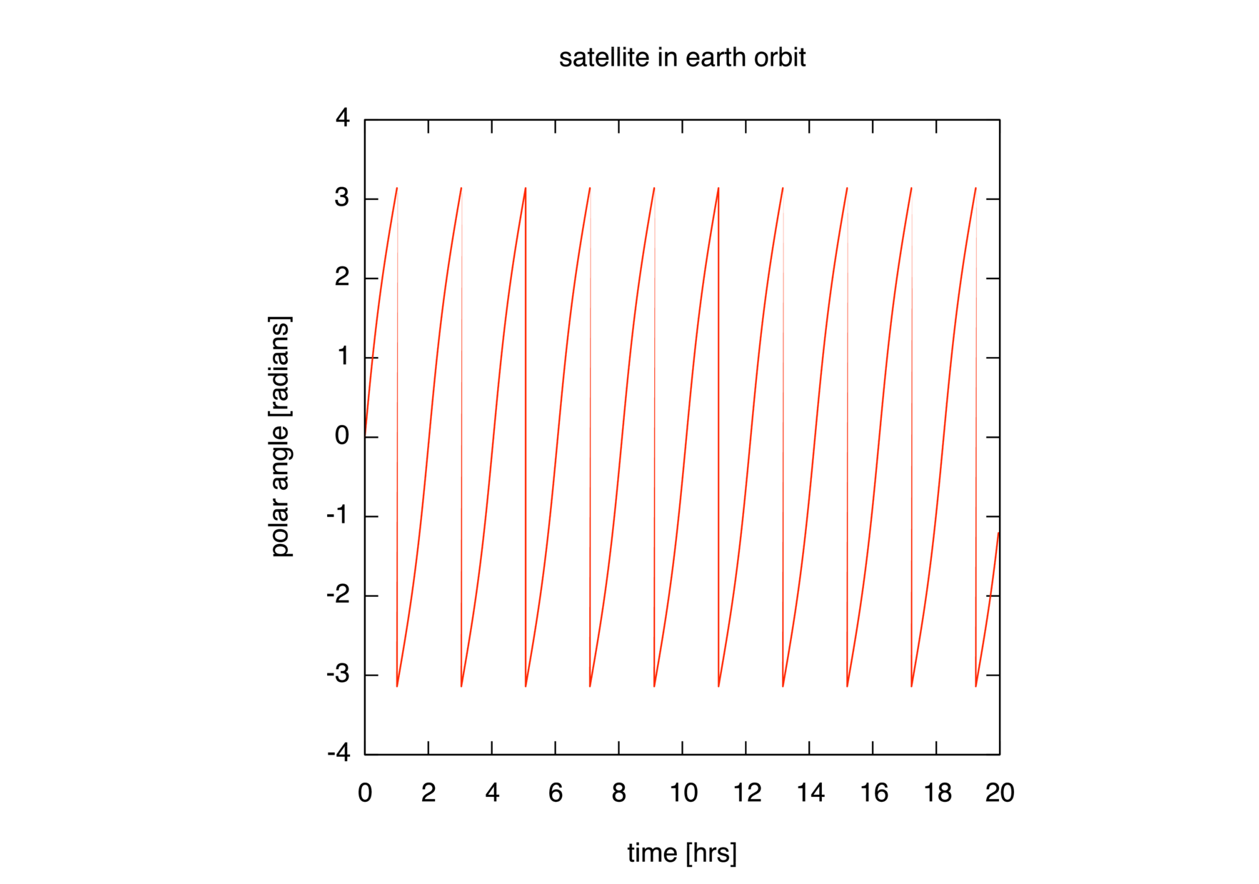
performed. The view1.gp script should give you the following
plots.
More eccentric still
Write a new program orbit_vel.cpp that functions identically to
orbit.cpp except that it outputs five columns of data: time
\(\mathsf{t}\), radius \(\mathsf{r}\), angle \(\theta\),
radial velocity \(\dot{\mathsf{r}}\), and angular velocity
\(\dot{\theta}\). The time derivatives \(\dot{\mathsf{r}}\) and
\(\dot{\theta}\) should be approximated as symmetric finite
difference. Some care must be taken in computing \(\dot{\theta}\)
since \(\theta\) is compact on \([\mathsf{0,2\pi}]\).
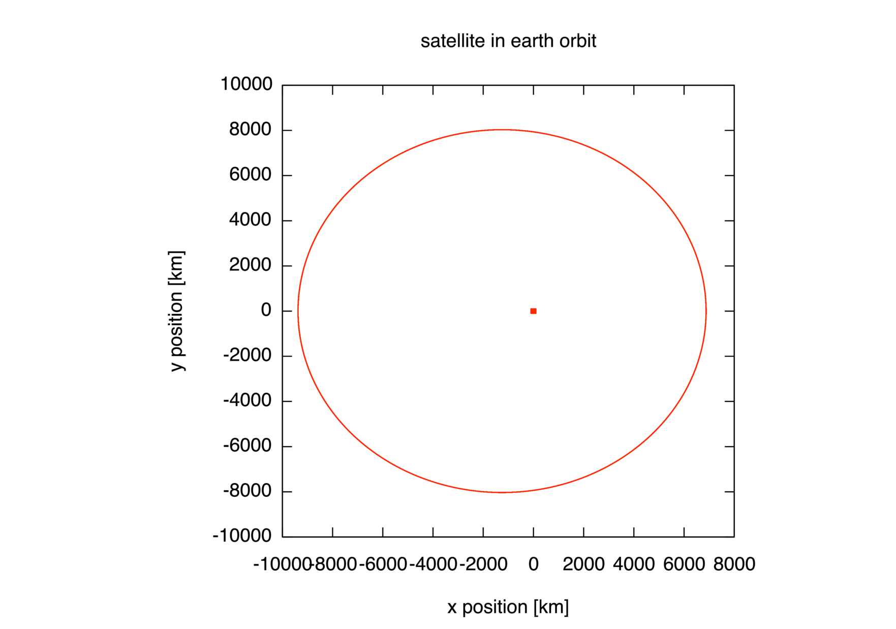
In orbit.cpp the closest- and farthest-approach values were set to
\(\mathsf{r_1} = \mathsf{R_{\textsf{e}}}
+ \mathsf{500}\,\textsf{km}\) and \(\mathsf{r_2}
= \mathsf{R_{\textsf{e}}} + \mathsf{3000}\,\textsf{km}\), where
\(\mathsf{R_\textsf{e}}\) is the radius of the earth. For
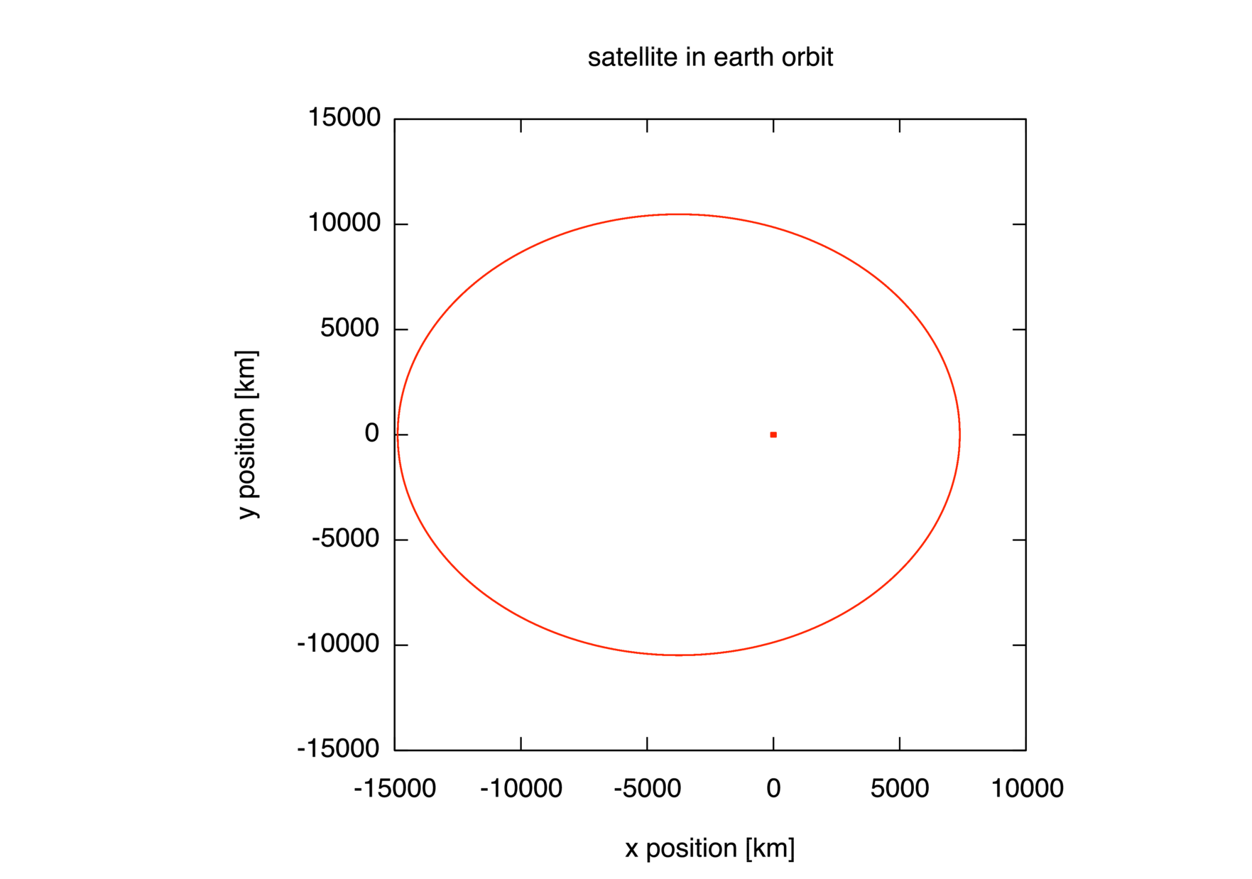
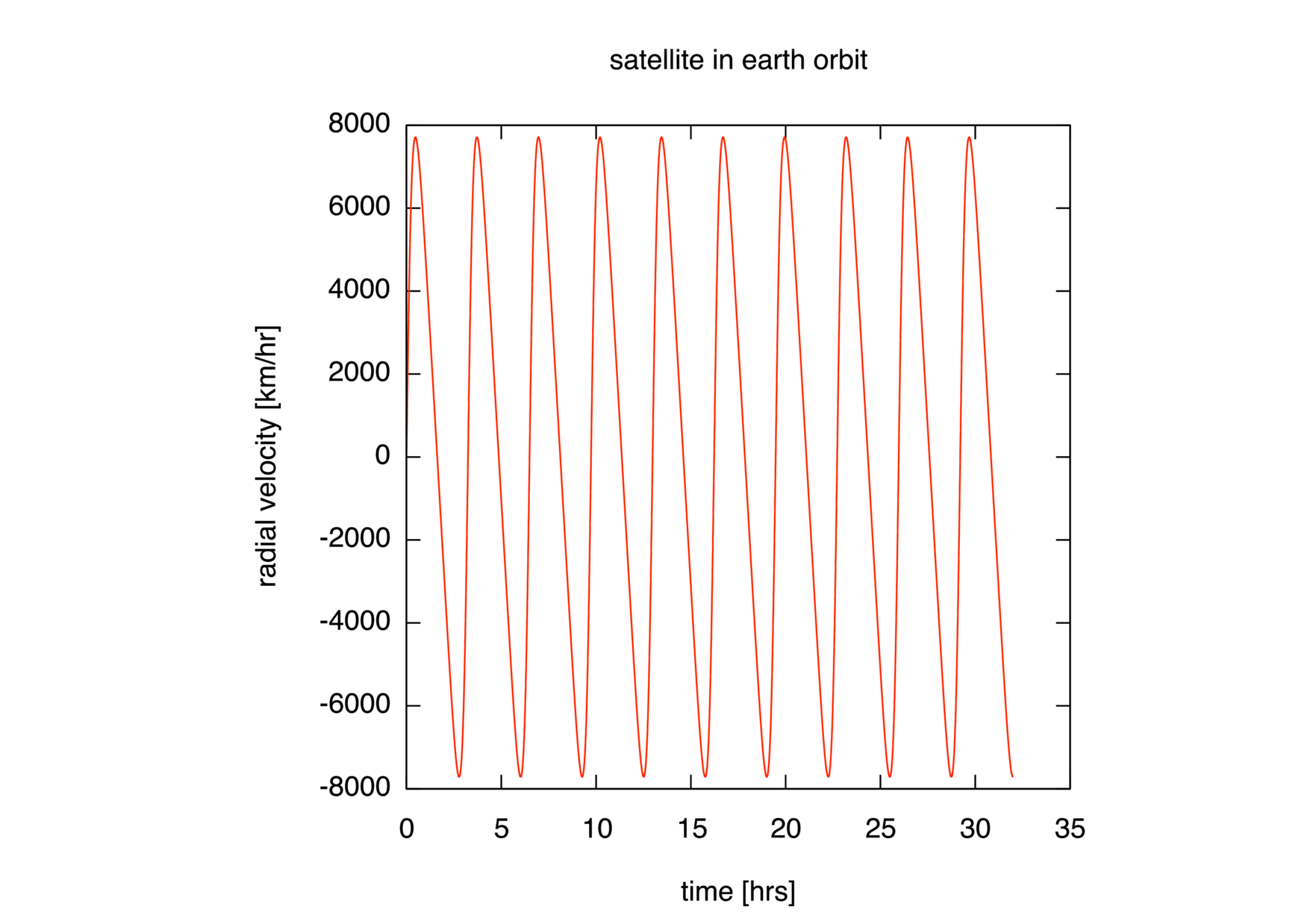
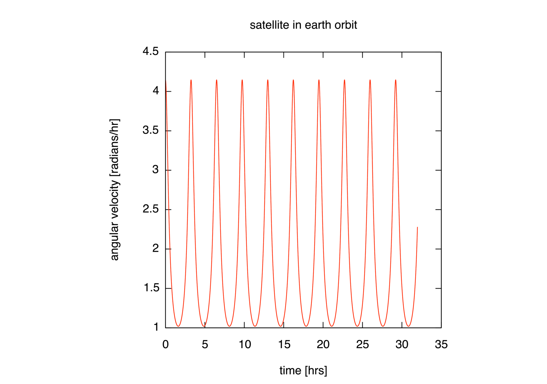
orbit_vel.cpp consider a more eccentric orbit with
\(\mathsf{r_1} = \mathsf{R_{\textsf{e}}}
+ \mathsf{1000}\,\textsf{km}\) and \(\mathsf{r_2}
= \mathsf{R_{\textsf{e}}} + \mathsf{8500}\,\textsf{km}\). Compose
a gnuplot script view2.gp that plots the satellite’s spatial
trajectory, its radial velocity versus time, its angular velocity versus
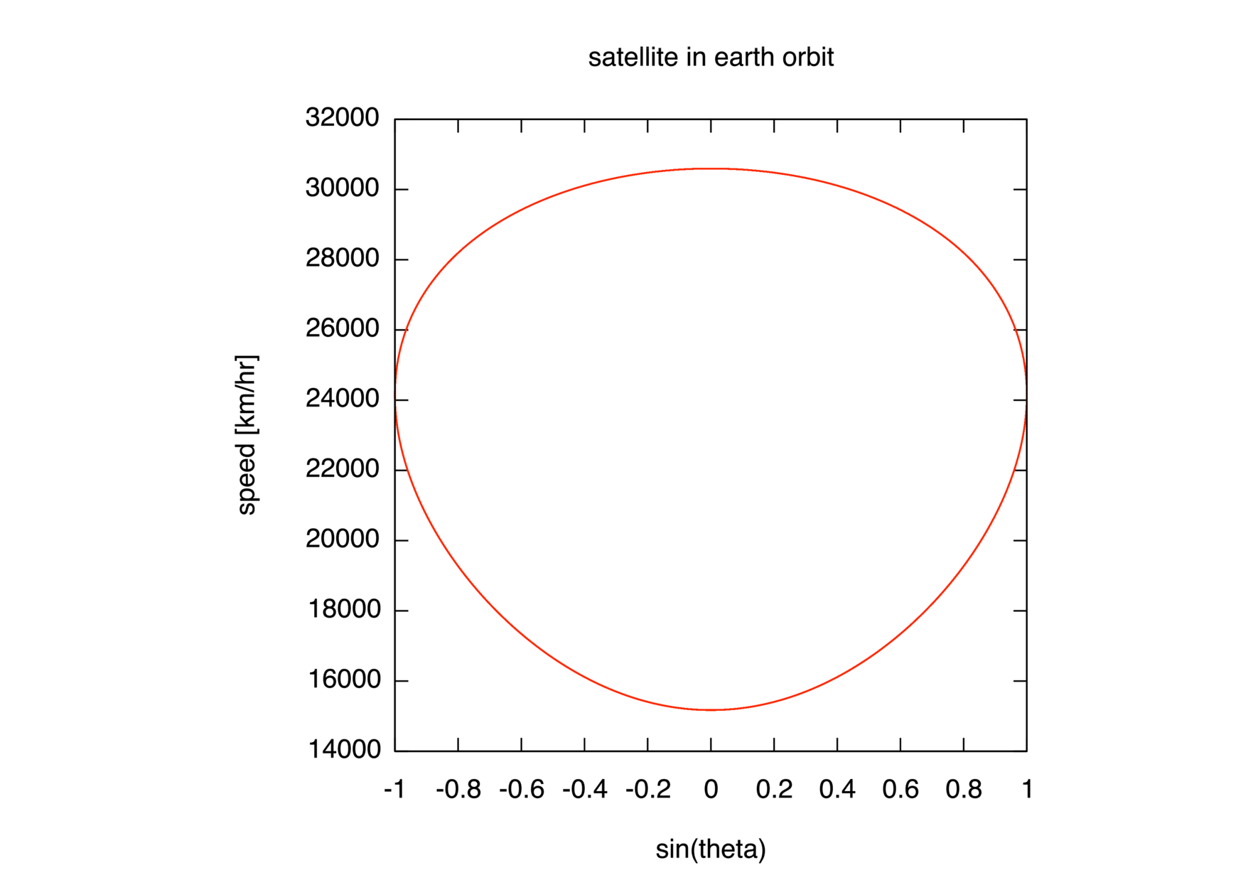
time, and its total speed versus \(\textsf{sin}\,\theta\), assuming
that the data is in a file ov.dat. (Arrange these as four plots in
succession, separated by a pause -1 command.) In the last plot, be
sure to compute the speed as the magnitude of the vector
\(\vec{\mathsf{v}}
= \dot{\mathsf{r}}\,\hat{\mathsf{r}} + \mathsf{r}\dot{\mathsf{\theta}}
\,\hat{\mathsf{\theta}}\).
$ make orbit_vel
$ ./orbit_vel > ov.dat
$ gnuplot -persist view3.gp
Square root by series expansion
Recall that Newton’s method is an iterative scheme for finding the zeros of an arbitrary function \(\mathsf{f(x)}\). It involves making an initial guess \(\mathsf{x_0}\) and then generating a sequence of improved estimates according to \(\mathsf{x_{n+1}} := \mathsf{x_n} - \mathsf{f(x_n)/f'(x_n)}\). If we choose \(\mathsf{f(x)} = \mathsf{x^2 - a}\), then finding the zeros of \(\mathsf{f(x)}\) is equivalent to computing the square root of \(\mathsf{a}\). The correct recurrence relation is
The program root.cpp implements the recurrence relation shown above,
starting from x = 1. The loop terminates when the next value in the
sequence is sufficiently close to the old one.
$ make root
g++ -o root root.cpp -O2 -ansi -pedantic -Wall -lm
$ ./root
Returns the square root of the provided argument:
Usage: root # [--verbose]
./root 2
Newton's method value: 1.414213562373095
 C Math library value: 1.414213562373095
$ ./root 9
Newton's method value: 3
 C Math library value: 3
$ ./root 101010
Newton's method value: 317.8207041713928
 C Math library value: 317.8207041713928
In general, computing square roots via series expansion is much less reliable, but let’s give it a try. The square root \(\sqrt{\mathsf{a^2+b}}\) can be expanded in powers of \(\mathsf{b/4a^2}\) as follows:
Here, \((\mathcal{C}_n) = (\mathsf{1}, \mathsf{2}, \mathsf{5}, \mathsf{14}, \mathsf{42}, \mathsf{132}, \mathsf{429}, \mathsf{1430}, \ldots)\) are the Catalan numbers. They are defined by
and describe the number of ways a polygon with \(\mathsf{n+2}\) sides can be cut into \(\mathsf{n}\) triangles. For large values of \(\mathsf{n}\), the factorials are too large to compute, so we should use the trick of computing each term from the previous one. The ratio of two consecutive terms is
Write a program seriesroot.cpp that computes the truncated
\(N\)-term series expansion for a given list of \(N\) values.
(In other words, argc can have any value greater than 3, and the
program should loop over all N assigned from argv[3],
argv[4], …, argv[argc-1].) You should be able to generate
the one- through ten-term approximations to \(\sqrt{\mathsf{2}}
= \sqrt{\mathsf{1^2+1}}\) and \(\sqrt{\mathsf{3}}
= \sqrt{\mathsf{2^2-1}}\) as follows. The script view3.gp illustrates
the convergence rates for Heron’s method and three different series
approximations to \(\sqrt{\mathsf{3}}\).
$ make seriesroot
g++ -o seriesroot seriesroot.cpp -O2 -ansi -pedantic -Wall -lm
$ ./seriesroot
Computes the N-term series expansion of sqrt(a^2+b):
Usage: seriesroot a b N1 [N2 N3 N4 ...]
$ ./seriesroot 1 1 $(seq 10)
             1                   1
             2                 1.5
             3               1.375
             4              1.4375
             5           1.3984375
             6          1.42578125
             7        1.4052734375
             8       1.42138671875
             9   1.408294677734375
            10   1.419204711914062
$ ./seriesroot 2 -1 $(seq 10)
             1                   2
             2                1.75
             3            1.734375
             4         1.732421875
             5    1.73211669921875
             6   1.732063293457031
             7   1.732053279876709
             8   1.732051312923431
             9   1.732050913386047
            10   1.732050830149092
$ gnuplot -persist view3.gp