Project 1

For a gas of particles of mass $\mathsf{m}$ in thermal equilibrium at temperature $\mathsf{T = 1/k_B\beta}$, the distribution of particle speeds $\mathsf{v = \lvert \mathbf{v} \rvert}$ is given by the famous Maxwell-Boltzmann distribution,

\[\mathsf{p(v) = \biggl(\frac{m \beta}{2\pi}\biggr)^{3/2}\!(4 \pi v^2) \, e^{-\beta m v^2/2}}.\]

The function $\mathsf{p(v)}$ is a probability distribution—meaning that $\mathsf{p(v)dv}$ is the probability of a given particle having a speed in the infinitessimal interval $\mathsf{[v,v+dv]}$—and the corresponding cumulative probability distribution is

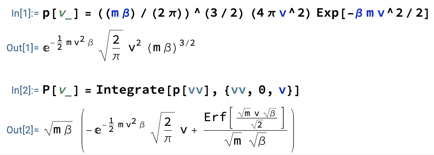
\[\mathsf{P(v) = \int_0^v\!dv'\,p(v') = \sqrt{m \beta} \Biggl(-\sqrt{\frac{2}{\pi}}\,v\, e^{-(\beta m/2) v^2} + \frac{1}{\sqrt{\beta m}} \text{Erf}\,\biggl[\sqrt{\beta m/2}\,v\biggr] \Biggr)}.\]

Try getting the latter from Mathematica:

p[v_] = ((m \[Beta])/(2 \[Pi]))^(3/2) (4 \[Pi] v^2) Exp[-\[Beta] m v^2/2]
P[v_] = Integrate[p[vv], {vv, 0, v}]

If we strip away all the dimensionful constants (setting $\mathsf{\beta m = 2}$, for instance), we lay bare the functional form:

$ gnuplot
> plot[0:5] (4/sqrt(pi)) * x**2 * exp(-x**2), -2/sqrt(pi) * x * exp(-x**2) + erf(x)

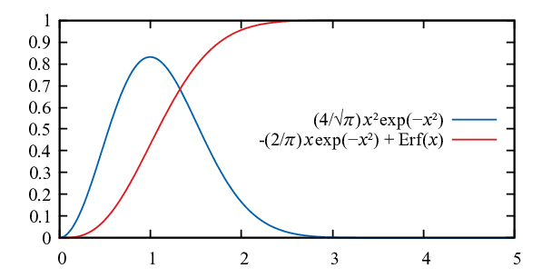
Note that $\mathsf{p}$ is everywhere non-negative, and hence $\mathsf{P}$ is monotonic non-decreasing; i.e., $\mathsf{p(v) \ge 0}$ implies $\mathsf{P(v_1) \le P(v_2)}$ for all $\mathsf{v_1 < v_2}$. Moreover, since $\mathsf{p}$ is as a probability distribution, it is normalized such that $\mathsf{\int_0^{\infty} \! dv\,p(v) = 1}$. This tells us that, as the speed ramps up from $\mathsf{v = 0}$, $\mathsf{P}$ grows from $\mathsf{P(0) = 0}$ and saturates at $\mathsf{\lim_{v\to\infty} P(v) = 1}$.

The correct way to randomly select a speed $\mathsf{v}$ from the distribution is to generate a pseudorandom variable $\mathsf{r \in [0,1)}$, drawn uniformly from the (left-closed, right-open) unit interval, and to match it ($\mathsf{0 \le r < 1}$) against the same value of the cumulative probability distribution ($\mathsf{0 \le P(v) < 1}$). Specifically, we generate a random $\mathsf{r}$ and compute the corresponding speed $\mathsf{v_r = P^{-1}(r)}$. But since, we don’t know the inverse function in this case—and it is very unlikely to have a neat, closed-form expression—we instead treat this as the problem of numerically identifying the (unique) value $\mathsf{v_r}$ such that $\mathsf{P(v_r) - r = 0}$. That is to say, we use a root finding algorithm.

The program mb.cpp computes the functions $\mathsf{p(v)}$ and $\mathsf{P(v)}$, in units where $\mathsf{m = k_B = 1}$, over a tight mesh of $\mathsf{v}$ values running from 0 to 10. These are output in three-column [$\mathsf{v}$, $\mathsf{p(v)}$, $\mathsf{P(v)}$] format to a file prob-distr.dat for each of temperatures $\mathsf{T = 1, 2, 3, 4, 5}$. The program is also meant to generate 1000 speed samples, drawn independently from the distribution $\mathsf{p(v)}$, for each of the five temperatures; these should be dumped to speed.dat. Your task here is to complete the empty function body of double newton_method(double, double, double), so that the program functions as intended. If your implementation of Newton’s algorithm is correct, you should be able to reproduce (with slightly different numbers, because of the randomness) the following terminal session:
```
$ cd project1/src-3d
$ make
g++ -o mb mb.cpp -O -std=c++20
$ ./mb
working on T = 1
working on T = 2
working on T = 3
working on T = 4
working on T = 5
$ ./speed-sort.bash
$ gnuplot speed.gp
Fitting the T = 1 data set
The best-fit parameter value:
 beta =  0.95715164213015 ± 0.000835298609062556

Fitting the T = 2 data set
The best-fit parameter value:
 beta =  0.48861480773466 ± 0.000402200896201479

Fitting the T = 3 data set
The best-fit parameter value:
 beta =  0.341789445311948 ± 0.000213286152445559

Fitting the T = 4 data set
The best-fit parameter value:
 beta =  0.247992859381509 ± 0.00013606506364919

Fitting the T = 5 data set
The best-fit parameter value:
 beta =  0.189675946323219 ± 0.000125834272739154
```
Explain in detail what the scripts speed-sort.bash and speed.gp are doing. Speculate as to why we’re not achieving fitted values that are exactly $\mathsf{\beta = 1, 1/2, 1/3, 1/4, 1/5}$.
Translate the mb.cpp program into either python or julia. In the case of python, you’ll want to import random in the preamble and call r = random.random() to assign a random number. In julia, the correct statement is r = rand(). Verify that your program produces properly formatted data files (*.dat) that feed correctly into prob-distr.gp, speed-sort.bash, and speed.gp.
Create a src-2d directory. Within that directory, redo the entire calculation for a two-dimensional gas of particles at temperatures $\mathsf{T = 1/2, 2, 4, 8}$. Use 4000 speed samples (quadruple what you used before). To obtain the correct Maxwell-Boltzmann distribution, simply replace the volumetric factor $\mathsf{(d/dv)(4/3)\pi v^3 = 4\pi v^2}$ with an areal factor $\mathsf{(d/dv)\pi v^2 = 2\pi v}$ and recompute the overall normalization to ensure that $P(\infty) = 1$. Show that the equation $\mathsf{P(v) = r}$ can be solved explicitly as $\mathsf{v = P^{-1}(r)}$ rather than applying numerical root-finding to $\mathsf{P(v) - r = 0}$. Generate the corresponding plots, and report the four temperature estimates extracted from fitting.