Assignment 3

Linear congruential generator

In class, we discussed the linear congruential generator scheme. Starting from a single initial seed \(\mathsf{x_0}\) (a non-negative integer), the sequence unfolds according to \(\mathsf{x_{n+1} = {(ax_n + c) \mod m}}\). The most convenient choice of modulus is \(\mathsf{m = 2^{64}}\), such that the modulus operation is effected automatically as overflow on a 64-bit fixed-width binary register.

In that case, if we take x to be of type UInt64, each next number in the sequence is found with a single multiplication and addition: x = a*x + c. The trick is to choose good values of the multiplier and increment. Two popular choices are shown in the table.

scheme	multiplier (\(\mathsf{a}\))	increment (\(\mathsf{c}\))
LLNL/SPRNG	2862933555777941757	3037000493
Knuth (MMIX)	6364136223846793005	1442695040888963407

These numbers are designed to satisfy the Hull–Dobell Theorem and thus ensure a repeat time of \(\mathsf{2^{64}}\), the maximum period. A known deficiency is that the least significant bits are somewhat less random than the most significant bits.

A convenient way to write this in Julia is with a closure, in which a function returns a function that captures a set of parameters provided by the user as arguments.

function create_lcg(a0, c0, x0)
   a = a0
   c = c0
   x = x0
   return function()
      x = a*x + c
      return x
   end
end

my_seed = UInt64(1975)
lcg = create_lcg(UInt64(2862933555777941757), UInt64(3037000493), my_seed)

# generate pseudorandom 64-bit sequences
lcg()
=> 0x8516d481892a6308
lcg()
=> 0x0ac522dfb57e5215
# interpret as signed, two's complement integers
reinterpret(Int64,lcg())
=> 712743970554937838
reinterpret(Int64,lcg())
=> -6940842903748281501
# rescale to produce numbers in the closed interval [0,1]
lcg()/(UInt64(0)-1)
=> 0.660163672390821
lcg()/(UInt64(0)-1)
=> 0.037941720613110005

Explain why the period of the linear congruential generator described above can never exceed \(\mathsf{2^{64}}\).

It’s sad/amusing to read about IBM’s RANDU generator, a notorious linear congruential generator developed by the company in the 1960s for use on its mainframes. It is widely considered one of the most flawed random number generators ever created. Many scientific results from that era that were based on Monte Carlo and stochastic methods are suspect.

Make an instance of RANDU using randu = create_lcg(UInt32(65539),UInt32(0), UInt32(seed))}. Generate 3000 numbers and output them to a file randu.dat in three-column format as follows:

\(\mathsf{x_0}\)	\(\mathsf{x_1}\)	\(\mathsf{x_2}\)
\(\mathsf{x_3}\)	\(\mathsf{x_4}\)	\(\mathsf{x_5}\)
\(\mathsf{x_6}\)	\(\mathsf{x_7}\)	\(\mathsf{x_8}\)
	\(\vdots\)
\(\mathsf{x_{2997}}\)	\(\mathsf{x_{2998}}\)	\(\mathsf{x_{2999}}\)

In gnuplot, type splot 'randu.dat' with points pointtype 7 pointsize 0.5, which can be abbreviated to splot 'randu.dat' w p pt 7 ps 0.5. Rotate the three-dimensional image until you can identify the flaw in the randomness. Include a screenshot or pdf of the revealing plot.

Manipulating floating-point representations at the bit Level

In Julia the reinterpret function can be used to read an integer’s bit pattern as a floating-point type. This is distinct from standard type casting, which tries to preserve value.

# Reinterpret the integer 4607182418800017408 as a Float64
UInt64(4607182418800017408)
=> 0x3ff0000000000000
Int64(0x3ff0000000000000)
=> 4607182418800017408
reinterpret(Float64, 0x3ff0000000000000)
=> 1.0
# On the other hand, casting gives
Float64(0x3ff0000000000000)
# = > 4.6071824188000174e18

Here, UInt64 and Float64 are the types we’d call unsigned long int (or uint64_t) and double in C++.

Recall that the 64-bit IEEE Standard 754 uses a bit pattern with 1 sign bit, 11 exponent bits, and 52 mantissa bits:

\(\mathsf{s}\)

\(\mathsf{e_{10}}\)

\(\mathsf{e_{9}}\)

\(\cdots\)

\(\mathsf{e_{0}}\)

\(\mathsf{m_{51}}\)

\(\mathsf{m_{50}}\)

\(\cdots\)

\(\mathsf{m_{0}}\)

Here, you will generate pseudorandom numbers in the range \(\mathsf{[0,1)}\). Furthermore, you will implement a shuffling scheme that renders the numbers more randomized. Start by populating an array num_bank with 1024 entries, each a 64-bit integer produced by a high-quality linear congruential generator. Once this initialization step is complete, carry out the following steps to produce the next number. Generate a 64-bit unsigned integer \(\mathsf{x = b_{63} b_{62} \cdots b_2 b_1 b_0}\). Ignore the two least significant bits (\(\mathsf{b_0}\) and \(\mathsf{b_1}\)). Harvest the next 10 bits to create a number \(\mathsf{k = 1 + b_{11}b_{10}\cdots b_4b_3b_2}\) (with \(\mathsf{1 \le k \le 1024}\)), which we will treat as a (one-based) array index. Swap the values of \(\mathsf{x}\) and the \(\mathsf{k}\!\) th element of num_bank. From the new \(\mathsf{x}\), create a floating point number \(\mathsf{1 \le f < 2}\) by transcribing the 52 most significant bits as follows:

\(\mathsf{0}\)

\(\mathsf{1}\)

\(\cdots\)

\(\mathsf{1}\)

\(\mathsf{b_{63}}\)

\(\mathsf{b_{62}}\)

\(\cdots\)

\(\mathsf{b_{14}}\)

\(\mathsf{b_{13}}\)

\(\mathsf{b_{12}}\)

Then return \(f-1\).

Examine the program shuffled-lcg.jl. Complete the missing return value so that each call to next_rnd() produces a floating-point number in the interval \(\mathsf{[0,1)}\) from the highest 52 bits in x following the shuffling scheme described above.

num_bank = Vector{UInt64}(undef, 1024)
for i in 1:1024
   num_bank[i] = lcg()
end

function next_rnd()
   x = lcg()
   k = x & ((1 << 12) - 1)
   k = (k >> 2) + 1
   # swap values
   num_bank[k], x = x, num_bank[k]
   return ????
end

All you need to report for this question is a valid Julia expression for the correct return value. Hint: my solution used the reinterpret function, a bit shift, a bitwise OR with a mask, and a floating-point subtraction.

There are various run tests that are used evaluate the apparent randomness of a pseudorandom sequence. Here is one scheme. For each number \(\mathsf{x}\), let \(\mathsf{x < 1/2}\) map to symbol “\(\mathsf{-}\)” and \(\mathsf{x \ge 1/2}\) map to “\(\mathsf{+}\)”. Then we can break up sequences \(\mathsf{(x_0, x_1, x_2, \ldots)}\) into contiguous runs of common symbols; e.g.

\[\mathsf{\underbrace{+ + +}_3 \overbrace{- - - - -}^5 \underbrace{+ + +}_3 - \underbrace{+ + + + + +}_6 - \underbrace{+ + +}_3}\]

shows 7 runs of size 3, 5, 3, 1, 6, 1, and 3. Prove that \(\mathsf{\textsf{Prob}(1\textsf{-run}) = 1/2}\), \(\mathsf{\textsf{Prob}(2\textsf{-run}) = 1/4}\), …, and \(\mathsf{\textsf{Prob}(n\textsf{-run}) = 2^{-n}}\).

Modify shuffled-lcg.jl so that it outputs a histogram of the frequency of \(\mathsf{n}\)-runs for \(\mathsf{n = 1, 2, \ldots, 20}\). You should be able to reproduce the terminal session below. For the two seeds shown, report the histogram entries for \(\mathsf{n = 5, 6, 7}\).

$ julia shuffled-lcg.jl
Usage: julia shuffled-lcg.jl <pseudorandom generator seed>
$ julia shuffled-lcg.jl 1975
1          0.5004000000
2          0.2484000000
3          0.1244000000
4          0.0657000000
.
.
20         0.0000000000
$ julia shuffled-lcg.jl 87263
1          0.5046000000
2          0.2529000000
3          0.1194000000
4          0.0607000000
.
.
20         0.0000000000

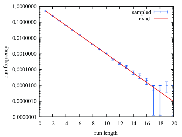
Generate \(\mathsf{N=20}\) such histograms, based on 20 different seeds. Collate the data sets to report the aggregate histogram in the format \(\mathsf{n}\), \(\mathsf{\textsf{AVE}[\textsf{Prob}(n\textsf{-runs})]}\), \(\mathsf{\textsf{ERR}[\textsf{Prob}(n\textsf{-runs})]}\), where \(\mathsf{\textsf{AVE}}\) denotes the mean over the \(\mathsf{N}\) instantiations and \(\mathsf{\textsf{ERR} = \sqrt{\textsf{VAR}/N}}\) is the square root of the variance from the mean divided by \(\mathsf{N}\).

By typing plot 'hist-all.dat' u 1:2:3 w e, 2**(-x) and then set logscale y; replot in gnuplot, you should be able to produce a plot similar to this: